3D Tokenizer Quality: SS + SLAT, and the codes-vs-cells law
All three discrete tokenizers (sparse-structure, shape, texture) on the frozen TRELLIS.2 VAE — and why each modality wants a different way to spend its token budget · 2026-06-25
The full 3D-token vocabulary is now three discrete tokenizers on the frozen TRELLIS.2 representations: SS (sparse structure / "where"), shape and texture SLAT ("what", on the structure). The headline finding: the two modalities want opposite ways to spend tokens.
The codes-vs-cells law: at a fixed token budget you can spend it on more spatial cells (finer grid, 1 code each) or more codes per cell (coarse grid, richer description). SS (a high-frequency occupancy boundary) wants more CELLS; SLAT (smooth features on a known surface) wants more CODES/cell.
SS: dense VQ-VAE on the (8,16³) latent. occ-IoU is brittle at 64³ but the SLAT only uses a 2× max-pooled 32³ structure — measured there, a VLM-affordable 12³ grid (1728 tok) reaches occ-IoU@32 ≈ 0.88.
SLAT (texture & shape): the winning config is 8³ × n_groups=4 (2048 tok) + ConvNeXt — more codes/cell, not more cells. At matched 150K/20k it beats the old VQ-1024 and even the old full-data baselines on feat-L1 (tex 0.414, shape 0.399).
Decode-space loss (material-L1 for texture, teacher-forced geom-decode for geometry) still applies on top; SS uses an occupancy-BCE decode loss at the 32³ supervision resolution.
Honest caveats: the SLAT codes-win comparison is confounded by params (the 8³ config is ~10× bigger than the grid config); and feat-L1 (latent) saturates while the decode-space metric keeps improving — judge on the decode metric + renders, not feat-L1.
1 · The three components & the budget question
A 3D object is generated coarse-to-fine: SS (a 64³ occupancy → defines which voxels exist) → shape/texture SLAT (32-ch features on those voxels). For a VLM to read & write 3D as tokens, each stage is its own discrete tokenizer. Per-object budget today: SS ≈ 1728 + shape 2048 + texture 2048 ≈ 5.8k tokens (≈ a high-res image).
For every tokenizer the same question arises: given N tokens, how do you arrange them in 3D? Two knobs:
n_groups (codes per cell): keep a coarse spatial grid (8³ = 512 cells), put k codes per cell → 512·k tokens. Each code adds bits to the description of a fixed coarse region.
grid (spatial cells): a finer grid (g³ cells), 1 code each → g³ tokens. More codes = finer spatial resolution, same bits per location.
2 · The codes-vs-cells law (the key finding)
Same total bit budget, two ways to spend it — and the right choice flips by modality:
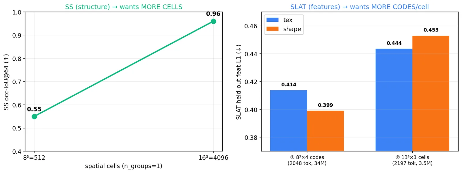
SS = the occupancy boundary itself (high spatial frequency). A code's 8³ cell covers an 8×8×8 region of 64³; one code can't say where the surface boundary sits inside it. So SS needs spatial resolution → more CELLS. 8³→16³ (same conv): occ-IoU@64 0.55→0.96, a huge architecture-independent jump.
SLAT = smooth features on an already-known surface (low frequency). The "where" is given by SS; SLAT only paints a smooth feature field, so it saturates spatially. Spending tokens on more CODES/cell (richer per-region description) wins. At matched ~2048 tokens: 8³×4 (codes) feat-L1 0.414/0.399 vs 13³×1 (cells) 0.444/0.453 — codes win on both tex & shape.
Intuition: cells buy spatial precision (where), codes buy descriptive richness (what). SS needs "where" → cells; SLAT needs "what" → codes. The two are mirror images.
Left: SS gains hugely from more spatial cells (8³→16³: 0.55→0.96 occ-IoU). Right: SLAT, at matched ~2048 tokens, is better with more codes/cell (8³×4) than more cells (13³×1). Opposite preferences.
3 · SS tokenizer (the new third component)
The SS latent is already dense (8, 16,16,16) — so the tokenizer is a plain dense 3D-conv VQ-VAE (no densify, no occupancy channel). The decode-space metric is occupancy: decode the recon latent through the frozen SS decoder → 64³ occupancy, compare to the GT-latent decode.
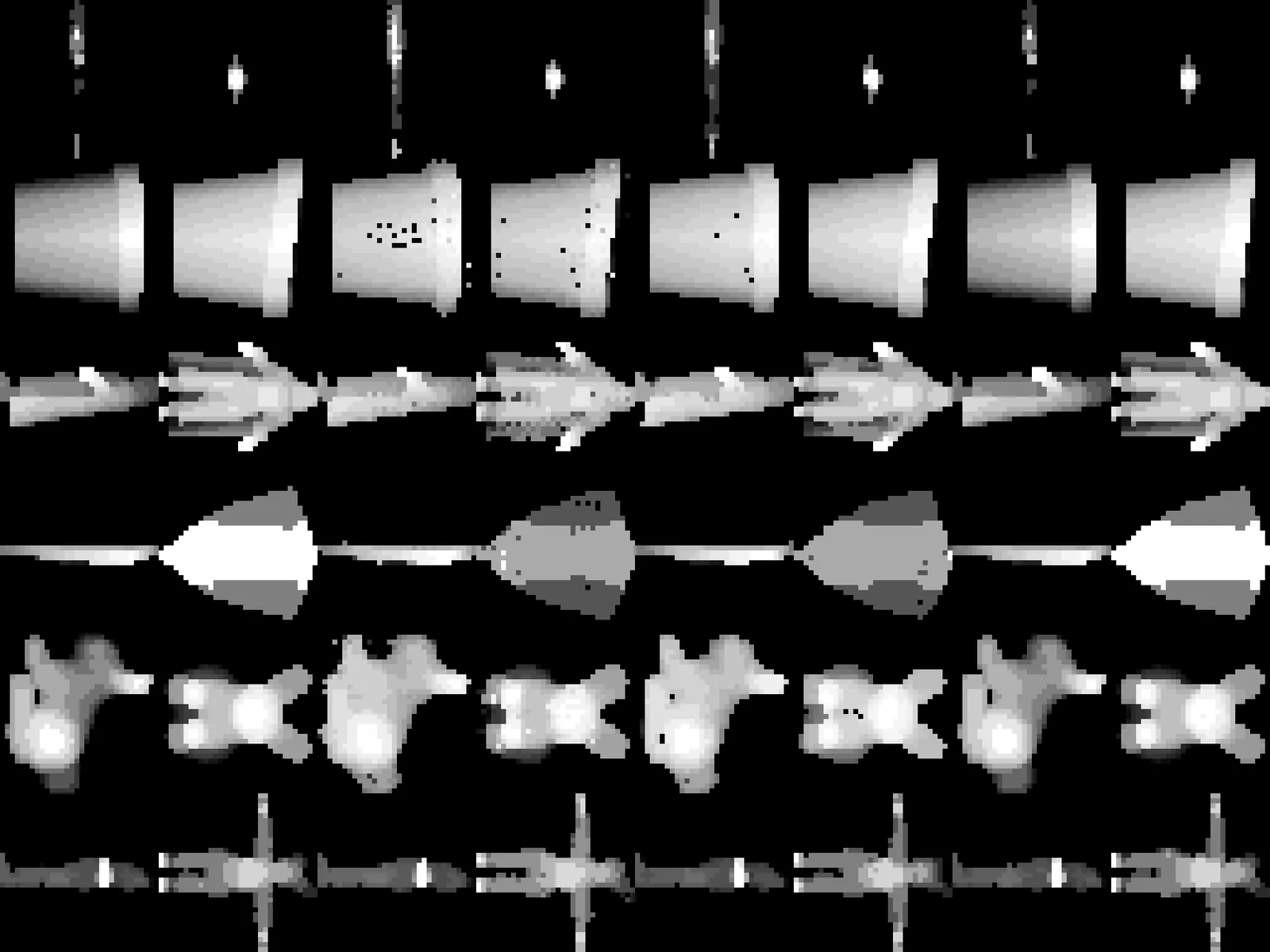
Measure at the right resolution. The pipeline never uses the 64³ occupancy directly — it max-pools 2× to 32³ to get the SLAT coordinates (verified in the TRELLIS pipeline code). occ-IoU@64 is brittle (a 1-voxel surface shift tanks it); occ-IoU@32 is what matters, and it's much higher.
SS config (full 490K, convnext, 32³-supervised)
tokens
occ-IoU@64
occ-IoU@32 (what SLAT uses)
8³ grid (1 code/cell)
512
~0.55
0.76
12³ grid (1 code/cell)
1728
—
0.88
16³ grid (2 codes/cell)
8192
0.96
0.98
1728 tokens (12³) is the VLM-affordable sweet spot at occ-IoU@32 ≈ 0.88. Near-lossless (0.98) needs 8192 tokens — too many for the VLM, and unnecessary once you measure at 32³.
SS reconstruction at 32³ (the SLAT resolution), held-out, depth-shaded projection (front|side): GT | 10³ 1000tok | 12³ 1728tok | 16³ 8192tok.
4 · SLAT winner: 8³ × n_groups=4 + ConvNeXt
Applying the codes-vs-cells law to SLAT: keep the 8³ grid, scale tokens via codes/cell (n_groups), and use the more-expressive ConvNeXt blocks (conv + per-voxel MLP, like TRELLIS's own SLAT VAE). At matched 150K data / 20k steps:
SLAT config (150K/20k)
mechanism
tokens
tex feat-L1
shape feat-L1
8³ × ng4, ConvNeXt
codes
2048
0.4137
0.3990
13³ × ng1, ConvNeXt (grid)
cells
2197
0.4435
0.4529
8³ × ng2, conv (old prod)
codes
1024
0.4496
0.4682
old full-data baseline
codes
1024
0.4188 (420K)
0.4381 (590K)
The 8³×ng4 ConvNeXt config at 150K already beats the old VQ-1024 at full data (tex 0.414<0.419, shape 0.399<0.438). Now scaling it to full data + the decode-space loss for the final checkpoints.
Caveat: the 8³ config (34M params) is ~10× bigger than the grid config (3.5M), so "codes win" is partly confounded by capacity; and the grid path also pays an interpolation cost. But the 8³×ng4 config beating the old full baselines makes it the practical winner regardless.
On top of the latent base, each component matches the frozen decoder's output, not the latent:
Texture → material-L1: decode recon & GT tex latents on the known geometry (shared guide_subs) → identical support → L1 on PBR voxels. (No rendering/LPIPS — that pushes the frozen decoder off-manifold.)
Geometry → geom-decode L1: the shape decoder predicts its own subdivisions, so supports differ (~45% overlap). Fix: capture the GT subdivisions, then teacher-force them on the recon decode (flip every pred_subdiv flag + pass guide_subs) → identical support → clean L1 on the 7-ch dual-grid output.
SS → occupancy-BCE at the 32³ supervision resolution (max-pool the decoder's 64³ occupancy to 32³, the resolution the SLAT actually consumes).
All decode-space losses lower decoded-output error while raising latent-fidelity metrics (occ-IoU/feat-L1) — that's the expected signature: the loss moves the latent off "best latent reconstruction" toward "best decoded output". Judge on the decode metric + renders.
6 · Final recipes (scaling to full data now)
component
latent
config
tokens
decode loss
key held-out metric
SS (structure)
dense (8,16³)
12³ grid · ng1 · ConvNeXt · more cells
1728
occ-BCE @32³
occ-IoU@32 0.88 ✅ full
Shape (geometry)
sparse SLAT 32³
8³ · ng4 · ConvNeXt · more codes
2048
geom-decode L1
geom-dec 1.539 (was 1.713, −10%) ✅ full
Texture
sparse SLAT 32³
8³ · ng4 · ConvNeXt · more codes
2048
material-L1
material-L1 0.0993 (was 0.1241, −20%) ✅ full
All three components are now full-data final checkpoints. The new SLAT config (8³×ng4 ConvNeXt + decode-loss) beats the previous VQ-1024 production: texture material-L1 0.1241 → 0.0993 (−20%), shape geom-decode 1.713 → 1.539 (−10%). One law, two opposite answers: SS spends its budget on cells (where), SLAT on codes (what).
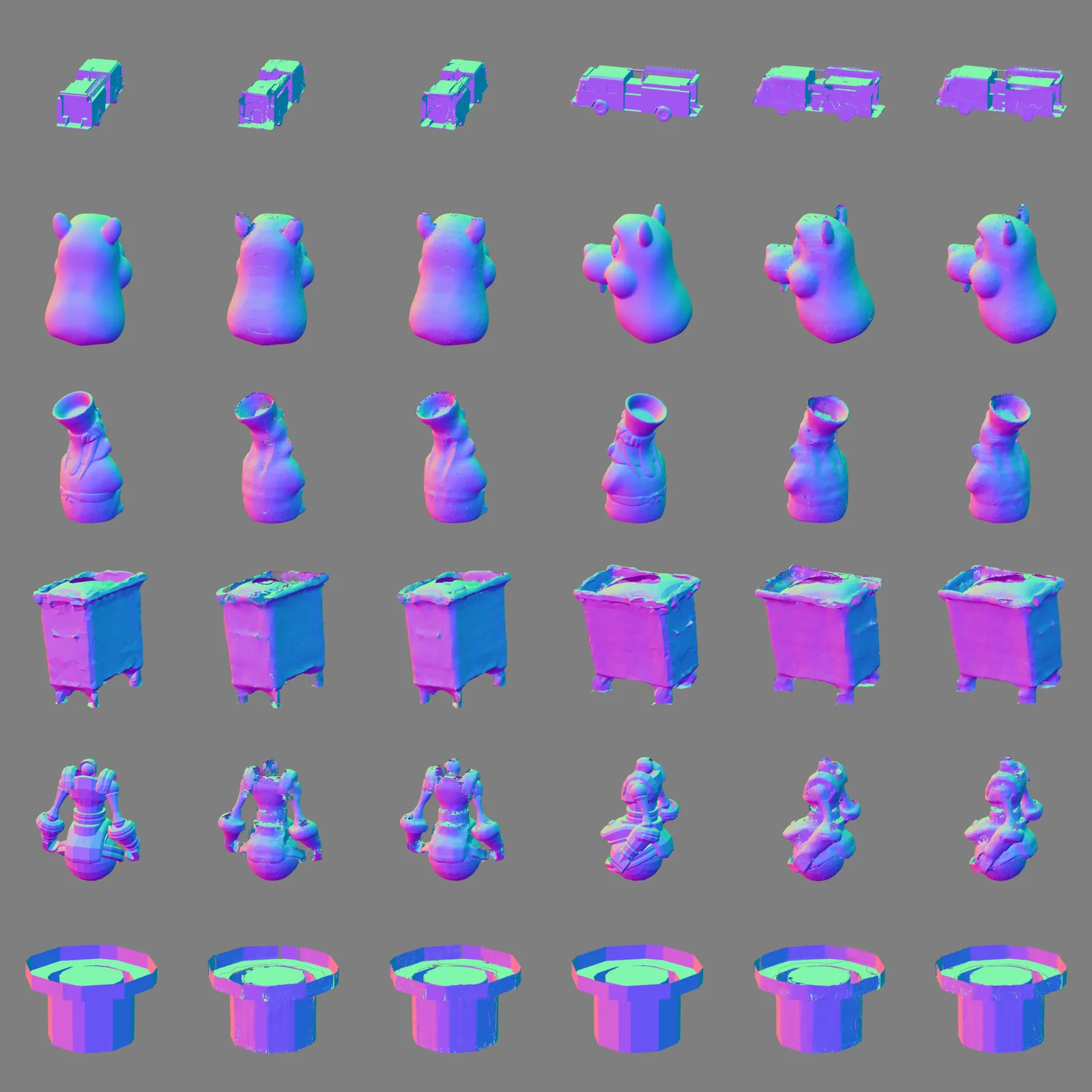
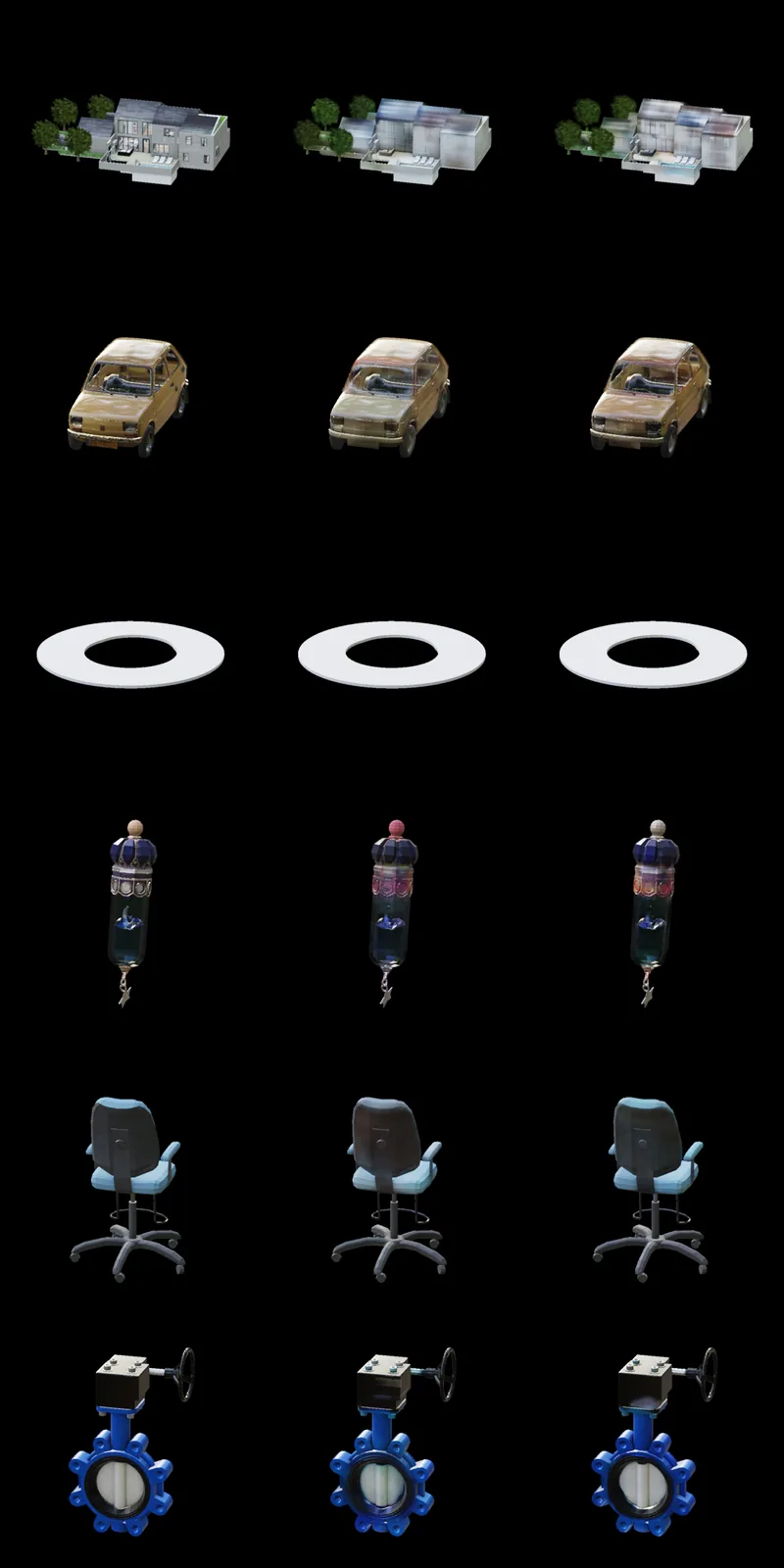
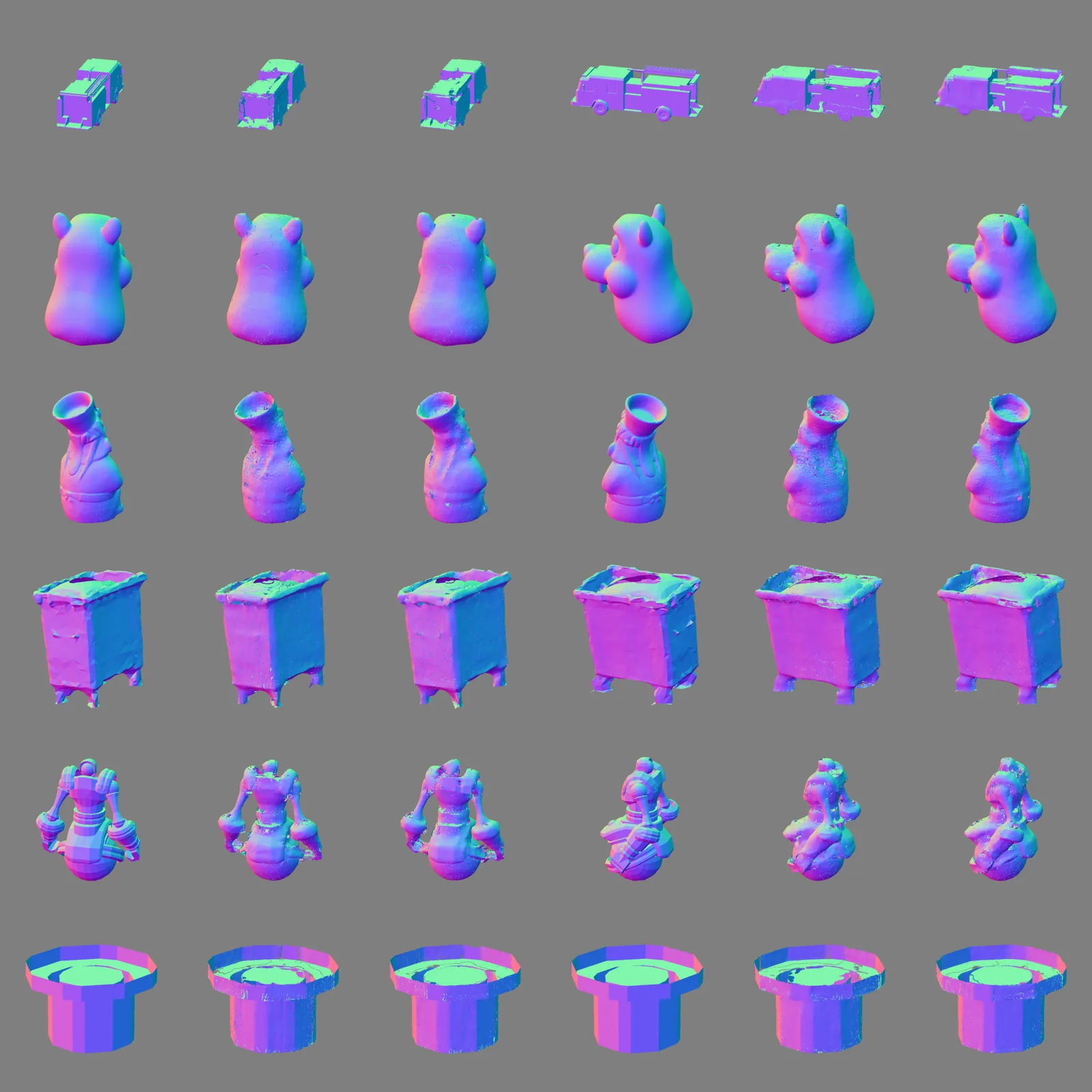
Final texture (held-out, envmap render): GT | old VQ-1024+material (1024 tok) | new 8³×ng4+material (2048 tok). material-L1 0.1241 → 0.0993.Final shape (held-out, normal maps): GT | old VQ-1024+geom (1024 tok) | new 8³×ng4+geom (2048 tok). geom-decode L1 1.713 → 1.539.
7 · Notes & open
Why the budget split: SS ≈ structure (high-freq) → cells; SLAT ≈ features on known geometry (low-freq) → codes. Falls straight out of rate-distortion + the signal's spatial frequency.
Metric discipline: feat-L1 (latent) saturates and misled an earlier "doubling doesn't help" call; the decode-space metric is the honest judge. Measure SS at 32³, not 64³.
Caveats to close: param-matched codes-vs-cells for SLAT; material-L1 (not feat-L1) on the 2048-token configs; full-data final checkpoints + decode losses (training now).
Next: finalize full-scale ckpts for all three; then VLM-side training (predict SS → shape → tex, coarse-to-fine).
8 · Held-out generalization & FSQ-vs-VQ (merged from the v1 FSQ→512 report, 2026-06-22)
The discrete tokenizer generalizes to held-out assets — the prerequisite for VP1 (a 3D-literate VLM): compress any TRELLIS.2 asset to a few hundred tokens/modality and decode back a faithful mesh + PBR on assets never seen during tokenizer training.
Held-out numbers (v1 FSQ→512, trained on all ready_v2 ~590K shape / ~420K PBR, 40K steps): shape feat-L1 0.466 / occ-IoU 0.915; texture 0.436 / 0.912. The 8³×n_groups=4 (2048-tok) config in §4 pushes feat-L1 further (shape 0.399, tex 0.414).
FSQ vs VQ: a naive VQ collapsed, but that was an implementation gap, not a VQ limitation — with standard stabilization a properly-engineered VQ is competitive. FSQ kept for simplicity/robustness.
repo weikaih04/slat-tokenizer · all comparisons same held-out assets · frozen decoders from TRELLIS.2 (2512.14692) · 2026-06-25